A Missing Generation: Comparison of U.S. Census Data (1900,2000)

A more interesting assignment from my Data Analysis and Visualization course at the University of Washington involved creating a static visualization of U.S. Census data from 1900 and 2000. Here's a sample of what we started with.

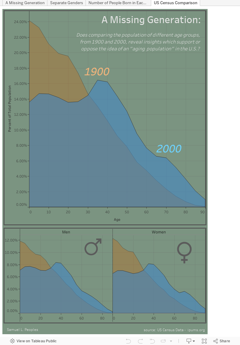
This visualization was approached with the question: “Does comparing the population of different age groups reveal insights which support or oppose the idea of an ['aging population'] in the United States?” With a few adjustments, the data can tell us a lot more than we think.

I began by encoding the Gender to “Men” and “Women”, and calculated the “Percent of Total Population” for each cell. This was accomplished by dividing each cell by the sum of all the values with the same “Year”. The year in which each age group was born was then calculated by subtracting the “Age” from the “Year”, and it was saved as “YearBorn” and used in the Tooltip.

Once all the necessary variables were assigned, I could then proceed with the analysis and comparisons. By standardizing the population with percentages, the differences in magnitude can be removed, although the individual values are immediately hidden. The differences between the genders is seemingly negligible, so it is appropriate to combine their values for a majority of the analysis.

When experimenting with different charts and graphs, the area graph was chosen to best represent the change in demography at these two snapshots in history. The most beneficial aspect of the area charts is that the shaded regions all sum to 100%, so direct comparisons can be made. The two graphs are overlayed upon one another and the stark differences can be seen, where blue and orange were used for their ability to capture attention, and help distinguish the two years from each other within the same chart. There is a significantly lower proportion of individuals born between 1965 and 2000, which does not follow the same trend as the rest of the visualization. This suggests that fertility rates significantly dropped around this time, and is supported by the fact that [oral contraceptives were first approved by the Food and Drug Administration in 1960]. This reduction has increased the median age of the United States, which is apparent from the space between the overlayed charts, where there are more individuals above the age of 40 comprising the total population in 2000, when compared to the proportion from 1900; this is roughly a constant three percent increase. This difference in proportion is taken from individuals under the age of 40, which is most apparent with the over ten percent difference of newborns, where this age group represented over twenty-four percent of the population in 1900, while they made up less than fourteen percent of the population by 2000.

Because the median age of the United States has increased and the representation of younger people in the national census has dramatically decreased, signs of an aging population can be observed. The use of area graphs to represent population proportions versus age is optimal for this question, where the true values are not immediately shown. However, hovering over points and selecting different portions of the visualization reveals these values, as well as information about when the age group was born, which helps guide the viewer through the data. This dataset is incredibly useful in the educational setting, where budding analysts are tasked with manipulating and contorting the data to reveal valuable insights. Initially viewing the data without standardization results in an opposing conclusion, which has the possibility of leading people to incorrect, or uninformed decisions. Although technology allows us to quickly analyze and understand huge datasets, it can be initially overwhelming, and exercises such as this are a great way to learn what does, and doesn’t work.

1. Select the different colored portions of the visualization. Does this change the information you can see?
2. Hover over the chart and describe the "Percent of Total" and number of people aged 40 in 1900, and 2000. Why is the population so much greater, when the proportion is lower?
3. What differences between individuals under 40 exist, and what does this suggest about the fertility rate of the United States?
4. In the area charts below, which gender appears to live the longest in the year 2000?
5. What is the general relationship between the genders?

[Here's a link to the dataset.]

Binary Classification of Titanic Survivors

I wanted to get some more machine learning practice down, and had heard about Trifacta in my Data Analysis and Visualization course, so I figured the [Titanic Kaggle exercise] would be fitting. I opted to use a Random Forest Classification, utilizing feature scaling and split training/ test data. The result left us with a model that was 84.93% accurate, with only 38 type I errors, and 25 type II errors, out of 418 samples.

The sinking of the RMS Titanic is one of the most infamous shipwrecks in history.  On April 15, 1912, during her maiden voyage, the Titanic sank after colliding with an iceberg, killing 1502 out of 2224 passengers and crew. This sensational tragedy shocked the international community and led to better safety regulations for ships.

One of the reasons that the shipwreck led to such loss of life was that there were not enough lifeboats for the passengers and crew. Although there was some element of luck involved in surviving the sinking, some groups of people were more likely to survive than others, such as women, children, and the upper-class.

In this challenge, we ask you to complete the analysis of what sorts of people were likely to survive. In particular, we ask you to apply the tools of machine learning to predict which passengers survived the tragedy.

So I began by taking a look at the data. Luckily, we were provided with three separate files.

• train.csv
• test.csv
• gender_submissions.csv

These files contain the relevant information for us to make the binary classification. Initially, we have some encoding, but our data is still quite messy. Our data arrived in the following format:

Variable	Definition	Key
survival	Survival	0 = No, 1 = Yes
pclass	Ticket class	1 = 1st, 2 = 2nd, 3 = 3rd
sex	Sex
Age	Age in years
sibsp	# Siblings / Spouses Onboard
parch	# Parents / Children Onboard
ticket	Ticket #
fare	Passenger Fare
cabin	Cabin number
embarked	Port of Embarkation	C = Cherbourg, Q = Queenstown, S = Southampton

Opening the datasets in Trifacta allows us to begin the preprocessing stage. Upon inspection of train.csv we can see that we have some missing values, as well as some mismatched values. Here, we'll take care of those, as well as drop unnecessary columns.

Because our datasets are ordered, and we want to create something we can work with, we'll remove the PassengerID column, as well as separate the Survived column into its own file, since our test data is already in that format.

I decided to separate my categorical variables using dummy variables, where I first worked with Pclass. I encoded the three columns into binary values, then removed a column to avoid the dummy variable trap. This left me with two boolean columns, one for First Class, and another for Third Class. The second replacement was for embarked; and here I made a difficult decision. I could have chosen to remove a column from my three choices between Cherbourg, Queenstown, and Southampton, but noticed that I had a fourth possibility, which was null. I opted to let null remain to be [0,0,0], while creating individual columns for Embarked_C, Embarked_Q, and Embarked_S. We'll see how that turns out. Finally, I one-hot encoded the Sex column, changing the name to Male to indicate that 1 was for Male, and 0 would be for Female.

I noticed that the columns for Cabin and Ticket were riddled with seemingly meaningless content, as well as dozens of missing values -- so we went ahead and dropped those too. Next we dealt with our numerical features, which were missing values for Age, and Fare. I opted to replace these missing values with the average across the columns, which will not affect the overall analysis.

Here's out it turned out:

The files were saved to their appropriate variables, ready to parse into Python.

• train_wrangled_X.csv
• tran_wrangled_y.csv
• test_wrangled.csv
• y_test_wrangled.csv

We begin by importing our libraries and datasets.

Next, I had noticed that some of our values ranged anywhere from [0,1] to [0,512], so I opted to include [feature scaling]. A downside here is that we, unfortunately, won't be able to see which features are having the most affect on our model, but this will improve our prediction, which is what we're aiming for anyway. The plus side to using feature scaling is that we reduce the possibility that one of our features will be overweighted in the algorithm, or if there is any codependency.

Now that our datasets are cleaned and ready to be modeled, we use the Random Forest Classifier, and predict our results. Here we choose ten estimators for our ten tested features, with the normal entropy and random state for recreation.

Finally, we test our results, finding a model that was 84.93% accurate, with only 38 type I errors, and 25 type II errors, out of 418 samples. I'd say that's pretty good accuracy!

Just for fun, I tried using this scaled and cleaned data in a dense neural network using Keras, which resulted in an accuracy of 90.19% I opted to use a softmax layer, which helps in the binary classification. After testing a few combinations of different activation functions, I was able to get the highest accuracy from this model, and felt pretty satisfied with the result.

If you want to check out the datasets, feel free to visit the github:
https://github.com/SLPeoples/Python-Excercises/tree/master/Titanic_Kaggle

Mushroom Classification with Keras and TensorFlow

Context

Although this dataset was originally contributed to the UCI Machine Learning repository nearly 30 years ago, mushroom hunting (otherwise known as "shrooming") is enjoying new peaks in popularity. Learn which features spell certain death and which are most palatable in this dataset of mushroom characteristics. And how certain can your model be?

Content

This dataset includes descriptions of hypothetical samples corresponding to 23 species of gilled mushrooms in the Agaricus and Lepiota Family Mushroom drawn from The Audubon Society Field Guide to North American Mushrooms (1981). Each species is identified as definitely edible, definitely poisonous, or of unknown edibility and not recommended. This latter class was combined with the poisonous one. The Guide clearly states that there is no simple rule for determining the edibility of a mushroom; no rule like "leaflets three, let it be'' for Poisonous Oak and Ivy.

• Time period: Donated to UCI ML 27 April 1987

I decided to give [this kaggle dataset] a shot. Here, we have over 8,000 samples of mushrooms which need to be modeled to determine whether or not they're edible. I used a Dense Neural Network to model and classify them, after encoding the variables and conducting a 75/25 training/test split. 

Here's how our data started. The following key can be used to understand the dataset entries.

• cap-shape: bell=b,conical=c,convex=x,flat=f, knobbed=k,sunken=s
• cap-surface: fibrous=f,grooves=g,scaly=y,smooth=s
• cap-color: brown=n,buff=b,cinnamon=c,gray=g,green=r,pink=p,purple=u,red=e,white=w,yellow=y
• bruises: bruises=t,no=f
• odor: almond=a,anise=l,creosote=c,fishy=y,foul=f,musty=m,none=n,pungent=p,spicy=s
• gill-attachment: attached=a,descending=d,free=f,notched=n
• gill-spacing: close=c,crowded=w,distant=d
• gill-size: broad=b,narrow=n
• gill-color: black=k,brown=n,buff=b,chocolate=h,gray=g,green=r, orange=o,pink=p,purple=u,red=e,white=w,yellow=y
• stalk-shape: enlarging=e,tapering=t
• stalk-root: bulbous=b,club=c,cup=u,equal=e,rhizomorphs=z,rooted=r,missing=?
• stalk-surface-above-ring: fibrous=f,scaly=y,silky=k,smooth=s
• stalk-surface-below-ring: fibrous=f,scaly=y,silky=k,smooth=s
• stalk-color-above-ring: brown=n,buff=b,cinnamon=c,gray=g,orange=o,pink=p,red=e,white=w,yellow=y
• stalk-color-below-ring: brown=n,buff=b,cinnamon=c,gray=g,orange=o,pink=p,red=e,white=w,yellow=y
• veil-type: partial=p,universal=u
• veil-color: brown=n,orange=o,white=w,yellow=y
• ring-number: none=n,one=o,two=t
• ring-type: cobwebby=c,evanescent=e,flaring=f,large=l,none=n,pendant=p,sheathing=s,zone=z
• spore-print-color: black=k,brown=n,buff=b,chocolate=h,green=r,orange=o,purple=u,white=w,yellow=y
• population: abundant=a,clustered=c,numerous=n,scattered=s,several=v,solitary=y
• habitat: grasses=g,leaves=l,meadows=m,paths=p,urban=u,waste=w,woods=d

The two surprising results that I found were actually really cool. First, I found that by using the Keras module, I did not need to one-hot encode my 22 categorical features. As seen in the encoding section below, just encoding the data was grueling enough, and I was not looking forward to separating them out and removing individual columns to control for dummy variables. What a relief! For each variable, the characters were encoded to numerical values, and the Neural network took it from there.

The second great finding was that the model completely trains with only one hidden layer in only twenty epochs! This means that the data is easily classified, but also suggests that the model should be tested on a completely independent dataset, just in case there is overfitting. Because the model is trained and tested on separate subsets of data, we can be fairly confident in our 100% accuracy.

Here's a link to the github:

https://github.com/SLPeoples/Python-Excercises/tree/master/MachineLearningPractice/02-Classification

If you're interested in the Nueral Network and how things came together, check out the Jupyter Notebook below!

Sentiment Analysis of Twitter Users

One of my soft spots is for social media, and how the public is influenced by it, so I decided to take a course in sentiment analysis using R and Tableau. The course exposed me to two lexicons which classify words as either "good" or "bad", which is really useful, since we can add or remove terms from the lexicons based on context. A good example would be the addition of local vernacular or industry conventions which wouldn't necessarily be universally negative or positive.

In this application, we looked at the sentiment and popularity of the Samsung Galaxy versus the Apple iPhone on Twitter from Los Angeles, New York, Austin, and Seattle. We scraped data from Twitter using R, after grabbing geocodes from https://www.latlong.net, which we passed through a sentiment function, and saved to individual output files. Check out the Jupyter Notebook below.




In Tableau, the extracted Tweets were joined into one data source for analysis. The first observation was that there was a very low number of Tweets in Seattle about Apple, even though the script was able to retrieve 2,000 entries for all other cities. This should be taken into consideration for all further insights.

The ratio of Original versus Duplicate Tweets was then analyzed, finding that 63.56% of the extracted tweets were duplicate entries, meaning that a majority of the discussion about the two products is being repeated in the cities sampled.

Of the Original Tweets, we noticed that 57.43% of them were Retweeted at least once.

Out of all the Tweets sampled, Samsung trailed Apple 44.58% to 52.52%, meaning that Apple is being discussed more than Samsung throughout the four cities Sampled.

A histogram of the Samsung and Apple sentiment was constructed. After removing neutral entries, it was readily apparent that although Apple is being discussed more, the sentiment of the Samsung histogram is more right-skewed, indicating that the discussion is more positive than that of Apple's. 89% of the Samsung data was positive, while only 68% of the Apple data was positive.

Visualizing the frequency of the Tweets for each of the devices show that they are both increasing during the two-week period of analysis, which may be a result of new devices being released, or any associated news releases surrounding either one of the companies. The two devices do seem to be competing based on the frequency graph, where the frequency of Tweets about Samsung and Apple are seemingly correlated to some degree.

Finally, a map was constructed displaying the distribution of total tweets between Samsung and Apple, showing that Apple clearly has dominance on Twitter, at least for the two-week sample period in Los Angeles, New York, Austin, and Seattle.

Here's a link to the github:

https://github.com/SLPeoples/Text-Mining-Sentiment-Analysis

Optimizing Digital Currencies

So if anyone else saw [John Geenty's article], you may be interested in this! I gave it a shot and had some nifty results.

The views contained in this post are my own and do not represent investment advise, the views of my employer or anyone else. This content is intended to be used and must be used for informational purposes only. It is very important to do your own analysis before making any investment based on your own personal circumstances. You should take independent financial advice from a professional in connection with, or independently research and verify, any information that you find in this post and wish to rely upon, whether for the purpose of making an investment decision or otherwise.

The following Jupyter Notebook describes a script which determines a low volatility, high returns portfolio between BTC, ETH, ETC, LTC, DASH, NEO, ZEC, and XMR. It uses sharpe ratios and data from the last three months, saves files to a timestamped folder, and creates png figure for reference. It will also print out the percent returns for the day for each digital currency and the average percent daily returns.


The information was then used to backtest the recommended model, as well as an aggressive model from the results. Given an initial investment of $1000.00 on 19 September 2017, the recommended portfolio would have grown to over $2100.00 during the three-month period, while the aggressive grows to over $3000.00 in value. Because of digital currencies being inherently volatile, the Sharpe ratios are less reliable than one would desire, but is a good metric for portfolio analysis in this case.

A safe conclusion to draw, regardless of discrete investment is that LTC and NEO are two low volatility, yet moderate-to-high returns currencies which should be monitored, while BTC and DASH are two highly variable currencies that have grown quickly in value over the last three months. Coupled with any other insights that can be drawn from the market, I think this was a very exciting exercise.

Recommended Portfolio Distribution (scatterPoints.csv [34607]):

• BTC: 0.0180410176875
• ETH: 0.00377590859407
• ETC: 0.00315474140452
• LTC: 0.366286372076
• DASH: 0.00114576353705
• NEO: 0.463456037585
• ZEC: 0.000253851426288
• XMR: 0.14388630769

Aggressive Portfolio Distribution(scatterPoints.csv [27989]):

• BTC: 0.51007444775
• ETH: 0.0123708535254
• ETC: 0.0872447919173
• LTC: 0.0907395166206
• DASH: 0.138406313313
• NEO: 0.08129648342
• ZEC: 0.0520898783671
• XMR: 0.0277777150871

Here's a link to the github:

https://github.com/SLPeoples/Python-Excercises/tree/master/CryptocurrencyOptimization

K Means Clustering of Mall Customer Data

As a part of the Udemy Machine Learning A-Z course, I got my hands dirty with a little K-Means clustering. The problem was fairly simple, where we received a sample of 200 customers of a local mall. This dataset contained information about customer gender, age, annual income, and spending score. We want to determine whether a customer is Careless, Sensible, Standard, Careful, or a Target for marketing campaigns due to their high income and high spending.

Within the Jupyter notebook below, the income and spending score were used to conduct the classification after noticing that the age and gender had no significant impact on the spending score. The "Elbow Method" was implemented to determine the optimal number of clusters for our analysis. In the visualization, a good choice looks to be five.

Once we've found our optimal number of buckets, the two chosen columns are fitted to the K-Means clustering algorithm.

We then visualize our predictions in Python, but ultimately decide that Tableau will more clearly describe our dataset.

Using the dashboard above, the customers can be clearly seen in their appropriate clusters. It's evident that the choice of five clusters was ideal, and that the "Target Customers" are well defined. I found this exercise to be really useful, and you're more than welcome to give it a shot! I've embedded the jupyter notebook below, and linked to the github as well.



github:
https://github.com/SLPeoples/Machine-Learning-A-Z/tree/master/Part%2004%20-%20Clustering/24_K_Means

Coal Terminal Maintenance Analysis

As a part of the Udemy Advanced Tableau course, I found the exercise described in the storyboard below really interesting. The course provided thorough explanation of the real-world example, and really exemplified how we can use data to solve problems that don't even exist yet.

https://public.tableau.com/profile/samuel.l.peoples#!/vizhome/CoalTerminalMaintenance_2/CoalTerminalMaintenanceAnalysis

The scenario is placed at a Coal Terminal in Australia, which has a series of machines processing the coal before it is loaded onto container ships. Since the ships are kept on a tight schedule, it's pretty noticeable why machine downtime would be a costly issue! Here, we're looking at only Stacker-Reclaimers (SR) and Reclaimers (RL).

The challenge was as follows:

You have been hired by a Coal Terminal to assess which of their Coal Reclaimer machine require maintenance in the upcoming month.

These machines run literally round the clock 24/7 for 365 days a year. Every minute of downtime equates to millions of dollars lost revenue, that is why it is crucial to identify exactly when these machines require maintenance (neither less or more frequently is acceptable).

Currently the Coal Terminal follows to following criterion: a reclaimer-type machine requires maintenance when within the previous month there was at least one 8-hour period when the average idle capacity was greater than ten percent. 

Your task is to find out which of the five machines have exceeded this level and create a report for the stakeholders with your recommendations.

So first, we needed to create a few table calculations for the idle capacity, and adjust the parameters to visualize the performance of the five machines for the past month in eight hour buckets. A red 10% threshold line was placed on each graph, clearly letting the viewer know whether the machines exceeded the idle capacity threshold. An orange trend line was also used to indicate whether the performance was constant, better, or worse, throughout the month.

Next each machine was individually analyzed, but first let's make a note of a few things. SR6 and RL2 seem to be in the same path, and it can be seen that SR6 exceeds the idle capacity threshold for quite a long period. This is a false positive because RL2 is operating at 100% of it's capacity during the same period, through having an idle capacity of zero. Another period to note is the missing data for SR1 and SR4A. This is accounted for because it can be assumed that the machines were stacking during this period, and thus would note be relevant to our analysis. This would however be something to verify with the client, as it is definitely has the potential to significantly skew the findings for the two machines.

So in conclusion, we can confidently say that RL1 should be flagged for maintenance, as it has exceeded the 10% idle capacity threshold four times, and has an increasing trend of under utilization.

SR4A should also be flagged for maintenance, where although it has not exceeded the 10% threshold, the high trend of under utilization will be more costly over time, and it will quickly exceed the idle capacity limit.

RL2, SR1 and SR6 are performing within standards, and should continue to be monitored for early signs the necessity for maintenance.

Using OpenCV to detect Faces and Smiles

As a part of a larger course on Computer Vision, I was exposed to some nifty applications of OpenCV. I was provided a pre-trained model which could identify faces and eyes, and was tasked with developing a way to detect smiles as an exercise.

After only a few lines of code, we are able to utilize the webcam and give the application a shot! With matplotlib, we are able to visualize the model in action.

With one simple edit, we are able to detect smiles, which really only detects the change in what the model sees as a "mouth" and matches the dimensions of the detected area to its pre-trained categorization for "smile".

The result is definitely enough to make you smile!

If you want to give this a shot, the Jupyter notebook is embedded below, as well as a link to the source code.


This is the first part of a Udemy Computer Vision course that I completed. The link to the github can be found here:

https://github.com/SLPeoples/Deep-Learning-and-Computer-Vision

Analysis of 1000 Startup Companies

As a part of a larger course on Tableau, I was exposed to some really exciting features of the program. In this scenario, an interactive dashboard was created in order to facilitate analysis of 1000 startup companies.

You have been approached by a Venture Capital Fund. The Board of Directors are currently reviewing 1000 potentially interesting startups and deciding on which ones they are going to invest in.

The criterion for selecting investments for this fund is a combination of:

• High revenue (2015) 
• Low expenses (2015)
• Top growth (2015)

Your task is to assist the Board in identifying which businesses represent the best investment opportunities.

In the visualization below, we'll accomplish the task set out in the scenario. We first notice that there is a Revenue versus Expenses scatterplot with some sliders and a reference legend, followed by a map which has similar coloring as the plot above.

Notice that the Expenses axis is reversed. This was done because it's much more intuitive to look for the desirable entries in the top-right of the figure, and since we are looking for high revenue, and low expenses, this layout accomplishes that goal.

Observe that the slider labeled "Growth Leaders" controls the shape and color of the top selected startup companies by Growth. This let's the viewer visualize their top performing investment opportunities.

We also see that there are two reference lines labeled "Revenue Cutoff" and "Expenses Cutoff". This allows the viewer to use the relevant sliders to control for their desired investment opportunities. We see that those companies that fall within the first quadrant (Upper-Right) are colored with a bright red, while those that fall outside are colored with a darker shade.

The map below allows the Venture Capital Fund visualize their potential investments, allowing them to take the geographic element into consideration. This is extremely helpful when making decisions between states with higher taxes or regulations, or when local economies are outperforming others within the nation.

With these features, the Board of Directors is able to take this sample of 1000 startups, and reduce their search to the Top 20 Startups by Growth, which is then further reduced to the Top 9 Startups by Growth with Expenses no greater than $5M, and Revenue no less than $9M. The interactive nature gets the viewer at the ground-level with the data, and guides them to well-founded, and pragmatic conclusions.

This dashboard was developed as the second part to a larger Udemy Advanced Tableau course. Here's a link to the github:
https://github.com/SLPeoples/Advanced-Tableau-DS

World Demographics Animation

I remembered seeing a very interesting visualization in my Engineering Statistics class. One which follows the relationship between fertility rate and life expectancy over time, showing how the demographics of third world countries are slowly approaching those of developed countries. That is, over time, the life expectancy of the global population is increasing, while fertility is decreasing. Check out this youtube video for more information!



So I grabbed some census data from the web, and tried to recreate what I saw above. Using Tableau made the problem ten times easier, as I only needed to aggregate the rows and columns with fertility rate, and life expectancy respectively, and add a page for each year. The result (after a little coloring) was actually really interesting! I made the animation into a gif using some free software, which displays pretty similar results when compared to the video above.

The workbook can be found here:

https://public.tableau.com/profile/samuel.l.peoples#!/vizhome/WorldDemographics_24/WorldDemographics

This post is part five of a larger Udemy Tableau Advanced course that I completed. The link to the github can be found here:

https://github.com/SLPeoples/Advanced-Tableau-DS

Tableau Visualization Sample

As an assignment for my Data Analysis and Visualization course at the University of Washington, we began by analyzing sample dashboards from the Tableau Public Gallery. In this example, we will be examining the correlation of customer ratings and experience across many industries.

Many businesses have survey data somewhere, waiting for better analysis. Using a survey containing ratings from 1 to 10, this analytical view correlates ratings of overall satisfaction, firm expertise, and likelihood to recommend for several customer segments. Each circle represents a segment defined by the combination of industry, job function, gender, and product. Size corresponds to the number of customers in that segment.
source: https://www.tableau.com/solutions/gallery/survey-satisfaction#phblP0m4Ai1Psl8F.99

Explore the dashboard above to answer the following questions:

1. What variables are being displayed in the graphs above? What changes occur when choosing a different industry or job function?
2. Does there seem to be a correlation between the "Length of Being Customer" and the rating scores for Recommendations, Satisfaction, and Expertise across all industries?
3. Which bucket of customers has the largest sample size?
4. For which industry do the most outliers exist?
5. How does the "Length of Being a Customer" affect the ratings across all industries?